Pysound changing frequency, amplitude, and offset of a sine wave
- Categories:
- pysound
In this example, we will change the frequency, amplitude, and offset of a sine wave. This is based on the article Creating a sine wave.
Changing the frequency
Here is the code:
from pysound.buffer import BufferParams
from pysound.oscillators import sine_wave
from pysound import soundfile
from pysound.graphs import Plotter

params = BufferParams()
out = sine_wave(params, frequency=250)
soundfile.save(params, 'sine-250.wav', out)
This works in the same way as the previous sine wave example, but we have set the frequency to 250 Hz in the sine_wave function. If you listen to the sound you will hear that it has a lower pitch.
Here is a graph of the sound:
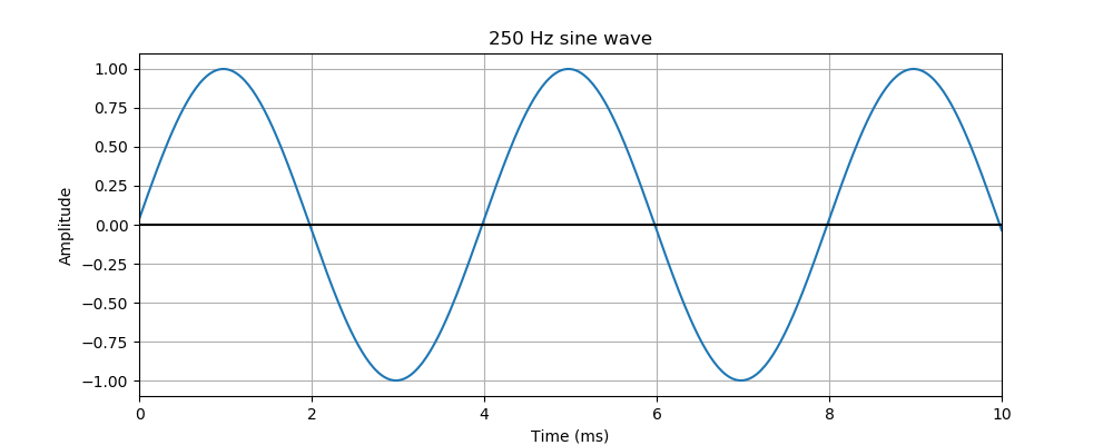
This shows the same 10 ms time range as the previous article, which showed a 500 Hz signal. For a 250 Hz signal, the wave period is one 250th of a second, ie 4 ms. This means that there will be 2.5 cycles in the 10 ms range of the graph.
The code to plot the graph is exactly the same as the previous article.
Changing the amplitude
Now we will see how to change the amplitude of the wave.
The default amplitude is 1.0, which means that the wave oscillates between the values +1.0 and -1.0, as you can see in the previous graph.
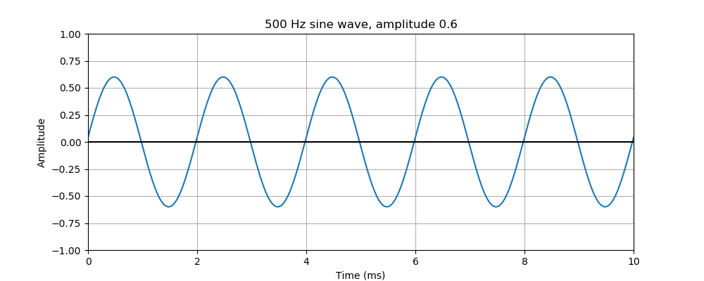
We will change the amplitude to 0.6, which means that the wave oscillates between the values +0.6 and -0.6. As you might imagine, this makes the sound a little quieter.
Here is the code:
out = sine_wave(params, frequency=500, amplitude=0.6)
soundfile.save(params, 'sine-500-6.wav', out)
In the sine_wave function, we have set the frequency back to 500 Hz and set the optional amplitude parameter to 0.6. Here is the graph:
Changing the plot scale
By default, when we plot a sound wave, Pysound sets the scale automatically to fit the wave. So when we plot a sound with an amplitude of 0.6, the graph will be adjusted so it has a range of +/- 0.6.
In this case, we want to compare this graph with the previous graph that had an amplitude of 1.0, so we want both graphs to be plotted with the same amplitude scale. We can do this by adding a call to with_yrange when we set up the plotting, like this:
## Plot a graph of the first part of the previous sine wave
Plotter(params, 'sine-500-6.png', out).with_timerange(0, 0.01)\
                                    .with_title("500 Hz sine wave, amplitude 0.6")\
                                    .with_yrange(-1, 1)\
                                    .in_milliseconds()\
                                    .plot()
Changing the offset
By default, the sine wave has an average value of zero. So if the amplitude is 0.6, it oscillates between +0.6 and -0.6.
It is sometimes useful to create a wave that oscillates about some other value. We can do that using the offset parameter. Here is an example:
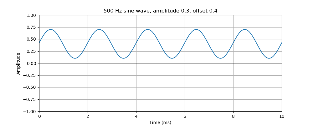
out = sine_wave(params, frequency=500, amplitude=0.3, offset=0.4)
soundfile.save(params, 'sine-500-3-4.wav', out)
In this case, the amplitude is 0.3 and the offset is 0.4, so the wave has the following characteristics:
- The maximum value is
offset + amplitude, or 0.7. - The maximum value is
offset - amplitude, or 0.1.
In other words, it is a sine wave of amplitude 0.3 that has been shifted up by 0.4
Here is the graph:
You can't hear this offset, in fact if you play the sound it is very likely that the audio amplifier will remove the offset altogether. However, the offset comes in very useful if you want to use the oscillator as a control signal, for example to create tremolo or vibrato effects.